1. Getting Started

In this project, we implement the Online Bayesian Inference algorithm for Collaborative Topic Regression model (obi-CTR) 2. The original CTR model 1 combines vanilla LDA 4 and PMF 6 for recommender systems. Although the CTR model has achieved good results in many fields, it is not suitable for online learning. Hence, Liu, Chenghao, et al proposed two models, the Online Decoupled Inference algorithm for CTR model (odi-CTR) and the obi-CTR model 2 for improving this issue. The former speeds up the fitting process by leveraging online LDA 5, which uses stochastic variational inference 8 technique. Despite speeding up, it performs relatively poorly on both rating prediction and topic modeling task, and it still needs to define the data size in advance, which is not a fully online learning fashion. On the other hand, the latter jointly optimizes the combined objective function of both LDA and PMF part. Moreover, by leveraging streaming variational Bayes 9, the obi-CTR model is fully online learning fashion. In addition, it uses hybrid strategy 7 to speed up. Among these three algorithms, the obi-CTR model consistently outperforms the others in most cases 2.

1.1. User Guide

In this section, we’ll guide you through the whole process of using the obi-CTR model, including initializing a ObiCTR object, fitting the model to the data and evaluating the performance of rating prediction and topic modeling task.

1.1.1. Initialization

The first thing to do is import the package and then initialize a ObiCTR object:

from recsys.ctr import ObiCTR
obj = ObiCTR(seed=1025)

1.1.2. Fitting the obi-CTR model

For the purpose of fitting a obi-CTR model to data, we load two sparse matrices, word count matrix, shape = (# items, vocabulary size) and rating matrix, shape = (# users, # items):

import scipy.sparse as sparse
word_cnt_mat = sparse.load(f"./data/word_count_mat.npz")
rating_mat = sparse.load(f"./data/rating_matrix.npz")

Then we feed the two sparse matrices to the model by invoking fit():

obj.fit(word_cnt_mat=word_cnt_mat, rating_mat=rating_mat)

It is worth noting that the model save all the fitted parameters automatically during the fitting process every evaluate_every times. Also, the model split ratings into two dataset, training data and validation data automatically, to evaluate the performance on validation data.

1.1.3. Evaluating RMSE and log likelihood

Once finished the fitted process, we can evaluate the performance of rating prediction task:

from recsys.utils.vec_utils import split_rating_mat
train_rating_mat, test_rating_mat = split_rating_mat(rating_mat=rating_mat, train_size=9000000, seed=1025)
obj.eval_rmse(rating_mat=test_rating_mat)

We can evaluate the performance of topic modeling as well:

obj.eval_avg_ll(rating_mat=test_rating_mat)

See eval_rmse() and eval_avg_ll() for more details.

1.1.4. Prediction

In obi-CTR model, rating prediction is defined as

\[\hat{r}_{ij} \triangleq \mathbb{E}[\mathbf{u}_i^{\top}\mathbf{v}_j].\]

It’s simply just the inner product of \(\mathbf{m}_{ui}\) and \(\mathbf{m}_{vj}\). For example, we can get the prediction of rating of item 5 given by user 3 by just calling predict_rating():

obj.predict_rating(user_id=3, item_id=5)

1.1.5. Updating parameters streamingly

Once finished the fitted process, we can fit the model to another mini-batch rating dataset:

obj.partial_fit(rating_mat=another_rating_mat)

See partial_fit() for more details.

1.1.6. Setting all the latent variables manually

It’s worth mentioning that we could also set all the fitted parameters manually by just feeding the correct data into set_vars():

# preparing all the fitted parameters...
# initialize a new object and set all the fitted parameters manually
another_obj = ObiCTR()
another_obj.set_vars(user_means=user_means, user_covs=user_covs,
                     item_means=item_means, item_covs=item_covs,
                     word_id_dict=word_id_dict,
                     topic_assignment_dict=topic_assignment_dict,
                     topic_word_mat=topic_word_mat)

After setting all the latent variables, another_obj is just like the fitted model and we could use it like we have mentioned before.

1.2. The obi-CTR Model in Depth

In this section we introduce the obi-CTR model in detail. Specifically, we talk about the mathematical concepts behind the model and how to implement it. Below is the graphical visualization of this probabilistic model:

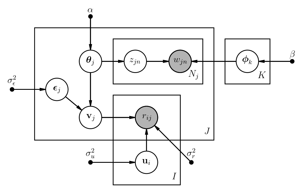
There are \(K\) topics, \(I\) users and \(J\) items, each item has \(N_j\) words. As you could see, the obi-CTR model is a high-dimensional model and the goal of it is to inference all the latent variables by just using relatively few observed variables. In our case, only parts of rating records and text content of each item are observed, while the rest are not. See the following information for a deeper understanding about each variable of this model.

Notations:

• \(\text{topic proportions:}~\boldsymbol{\theta}_j \sim \text{Dirichlet}(\alpha)\)

• \(\text{topic:}~\boldsymbol{\phi}_k \sim \text{Dirichlet}(\beta)\)

• \(\text{topic assignment:}~z_{jn} \sim \text{Multinomial}(1,~\boldsymbol{\theta}_j)\)

• \(\text{word:}~w_{jn} \sim \text{Multinomial}(1,~\boldsymbol{\phi}_{z_{jn}})\)

• \(\text{item latent offset:}~\boldsymbol{\epsilon}_j \sim \text{N}(\mathbf{0},~\frac{1}{\sigma_{\epsilon}^2}\mathbf{I}_K)\)

• \(\text{item latent vector:}~\mathbf{v}_j = \boldsymbol{\epsilon}_j + \boldsymbol{\theta}_j \sim \text{N}(\boldsymbol{\theta}_j,~\frac{1}{\sigma_{\epsilon}^2}\mathbf{I}_K)\)

• \(\text{user latent vector:}~\mathbf{u}_i \sim \text{N}(\mathbf{0},~\frac{1}{\sigma_{u}^2}\mathbf{I}_K)\)

• \(\text{rating:}~r_{ij} \sim \text{N}(\mathbf{u}_i^{\top}\mathbf{v}_j,~ \frac{1}{\sigma_{r}^2}\mathbf{I}_K)\)

1.2.1. Generative process

The generative process of the obi-CTR model is as follows:

1. For each user \(i\), draw user latent vector \(\mathbf{u}_i\).

2. For each topic \(k\), draw topic \(\boldsymbol{\phi}_k\).

3. For each item \(j\):

1. Draw topic proportions \(\boldsymbol{\theta}_j\).

2. Draw item latent offset \(\boldsymbol{\epsilon}_j\) and set item latent vector \(\mathbf{v}_j = \boldsymbol{\epsilon}_j + \boldsymbol{\theta}_j\).

3. For each word position \(n\) in item \(j\):

1. Draw topic assignment \(z_{jn}\).

2. Draw word \(w_{jn}\).

4. For each user-item pair \((i,~j)\), draw rating \(r_{ij}\).

1.2.2. Mathematical techniques and implementing the core algorithm

First, the obi-CTR model leverages streaming variational Bayes 9 to relax the assumption that the data size must be defined in advance. In particular, suppose the training data \(\mathbb{x}_1,\mathbb{x}_2,\dots\) are generated i.i.d. according to a distribution \(p(\mathbb{x}|\Theta)\) given parameters \(\Theta\), and we have seen and processed \(T-1\) samples \(\{\mathbb{x}_t\}_{t=1}^{T-1}\). Then Bayes theorem gives us the posterior after observing \(T\) samples

\[p(\Theta | \mathbb{x}_1, \dots,\mathbb{x}_T) \propto p(\mathbb{x}_T|\Theta)p(\Theta | \mathbb{x}_1, \dots, \mathbb{x}_{T-1})\]

That is, we treat \(p(\Theta | \mathbb{x}_1, \dots, \mathbb{x}_{T-1})\) as the new prior for the incoming data point \(\mathbb{x}_T\).

Moreover, there are two ways to implement approximate inference of the Bayes networks, variational inference (VI) (4, 5, 8, 9) and Markov Chain Monte Carlo (MCMC) 3. The obi-CTR model uses hybrid strategy 7 to get the approximate sufficient statistics of variational parameters of each “topic” dirichlet distribution and each “item latent vector” normal distribution. Specifically, we run gibbs sampling \(S\) rounds to draw new topic assignments. After \(B\) burn-in sweeps, we use rest samples to update. In addition, it allows us not to represent topic proportions \(\boldsymbol{\theta}_j\) and we can calculate \(k\)-th element of the topic proportions

\[\boldsymbol{\theta}_j^k=\dfrac{\mathbf{C}_j^k + \alpha}{\sum_{k=1}^K \mathbf{C}_j^k + K \alpha}\]

where \(\boldsymbol{\theta}_j^k\) is \(k\)-th element of topic proportions \(\boldsymbol{\theta}_j\) and \(\mathbf{C}_j^k\) is the number of words in item \(j\) that are assigned to topic \(k\) and \(\mathbf{C}_j=(\mathbf{C}_j^1,~\dots,~\mathbf{C}_j^K)\).

Furthermore, inspired by supervised topic model 10, \(\mathbf{v}_j\) is set to \(\boldsymbol{\epsilon}_j + \bar{\mathbf{z}}_j\) where \(\bar{\mathbf{z}}_j=\frac{\mathbf{C}_j}{N_j}\) is empirical topic frequencies of item \(j\), instead of the original setting, for simplifying the mathematical inference.

Finally, below is the summary of the implementation of the obi-CTR model:

1. Randomly initialize

• \(\{(\mathbf{m}_{ui},~\Sigma_{ui})\}_{i=1}^{I}\), variational parameters of each user latent vector \(\mathbf{u}_i\), and

• \(\{(\mathbf{m}_{vj},~\Sigma_{vj})\}_{j=1}^{J}\), variational parameters of each item latent vector \(\mathbf{v}_{j}\), and

• \(\{\mathbf{z}_j\}_{j=1}^{J}\), topic assignment of each word \(w_{jn}\) in each item \(j\) where \(\mathbf{z}_j = \{ z_{jn} \}_{n=1}^{N_j}\).

2. Receive a new data sample:

• \(r_{ij}\), rating of item \(j\) given by user \(i\), and

• \(\mathbf{w}_j\), text content of item \(j\) where \(\mathbf{w}_j=\{w_{jn}\}_{n=1}^{N_j}\).

3. For each gibbs sampling round \(s\):

1. For each word \(w_{jn}\) in item \(j\):

1. Draw new topic assignment \(z_{jn}^s \sim q(z_{jn}^s | \cdots)\) in round \(s\).

2. If \(s>B\), then collect \(z_{jn}^s\).

4. For each word \(w_{jn}\) in item \(j\), use collected samples \(\{z_{jn}^s\}_{s=S-B}^S\) to estimate \(\gamma_{jn}^k\), the probability of assigning word \(w_{jn}\) to each topic \(k\).

5. Update \(\{\Delta_k\}_{k=1}^{K}\), variational parameters of each topic \(\boldsymbol{\phi}_k\).

6. Update

• \((\mathbf{m}_{ui},~\Sigma_{ui})\), variational parameters of user latent vector \(\mathbf{u}_i\), and

• \((\mathbf{m}_{vj},~\Sigma_{vj})\), variational parameters of item latent vector \(\mathbf{v}_j\).

7. Repeat step (2), (3), (4), (5), (6).

1.3. Mathematical Formulation

1.3.1. Draw topic assignments

New topic assignment can be drawn from the conditional distribution of one variable \(z_{jn}\) given others:

\[\begin{split}\begin{aligned} q&(z_{jn}=k | \mathbf{z}_{j \lnot n} ,~ \mathbf{v}_j ,~ \Phi ,~ w_{jn}) \\ &\propto \underbrace{(\alpha + \mathbf{C}_{j \lnot n}^{k}) \exp \Bigg(\Lambda_k,w_{jn}}_ {\text{LDA part}} + \underbrace{\dfrac{1}{2 \sigma_{\epsilon}^2 N_j} \Big(2 \mathbf{m}_{vj}^{k} - \dfrac{1 +2 \mathbf{C}_{j \lnot n}^{k}}{N_j} \Big)}_ {\text{PMF part}}\Bigg) \end{aligned}\end{split}\]

See 2 in detail.

1.3.2. Update variational parameters of topics

Update variational parameters of topic \(\boldsymbol{\phi}_k\):

\[\Delta_{kw}^{\star} = \Delta_{kw}^{t} + \sum_{n=1}^{N_j}\gamma_{jn}^k \mathbb{I}[w_{jn}=w]\]

where \(\gamma_{jn}^k\) is the probability of assigning word \(w_{jn}\) to topic \(k\), which is estimated from the samples drawn from previous gibbs sampling process.

See 2 in detail.

1.3.3. Update variational parameters of user latent vector

Update the mean vector of user latent vector \(\mathbf{u}_i\):

\[\mathbf{m}_{ui}^{*} = \mathbf{m}_{ui}^{t} + \dfrac{r_{ij} - \mathbf{m}_{vj}^{\top} \mathbf{m}_{ui}^{t}} {\sigma_r^2 + \mathbf{m}_{vj}^{\top} \Sigma_{ui}^{t} \mathbf{m}_{vj}} \Sigma_{ui}^{t} \mathbf{m}_{vj}\]

Update the covariance matrix of user latent vector \(\mathbf{u}_i\):

\[\Sigma_{ui}^{*} = \Bigg( \big( \Sigma_{ui}^t \big)^{-1} + \dfrac{\mathbf{m}_{vj}\mathbf{m}_{vj}^{\top}} {\sigma_{r}^2 \mathbf{I}_{K}} \Bigg)^{-1}\]

See 2 in detail.

1.3.4. Update variational parameters of item latent vector

Update the mean vector of item latent vector \(\mathbf{v}_j\):

\[\mathbf{m}_{vj}^{*} = \underbrace{\color{red}{\Sigma_{mix} \Sigma_{vj}^{-1} \mathbf{m}_{vj}^{t}}}_ {\color{red}{\text{red}}} + \underbrace{\color{green}{\Sigma_{mix} \dfrac{1}{\sigma_{\epsilon}^2} \bar{\mathbf{z}}_j}}_ {\color{green}{\text{green}}} - \underbrace{\color{blue}{\Sigma_{mix} \dfrac{1}{\sigma_{r}^2} \mathbf{m}_{ui}}}_ {\color{blue}{\text{blue}}} \Bigg( \dfrac{\mathbf{m}_{ui}^{\top} \color{red}{\text{red}} + \mathbf{m}_{ui}^{\top} \color{green}{\text{green}} - r_{ij} }{ 1 + \mathbf{m}_{ui}^{\top} \color{blue}{\text{blue}} } \Bigg)\]

where \(\Sigma_{mix} = \big( \Sigma_{vj}^{-1} + \frac{1}{\sigma_{\epsilon}^2} \big)^{-1}\).

Update the covariance matrix of item latent vector \(\mathbf{v}_j\):

\[\Sigma_{vj}^{*} = \Bigg( \big( \Sigma_{vj}^{t} \big)^{-1} + \dfrac{1}{\sigma_{\epsilon}^2 \mathbf{I}_{K}} + \dfrac{\mathbf{m}_{ui} \mathbf{m}_{ui}^{\top}} {\sigma_{r}^2 \mathbf{I}_{K}} \Bigg)^{-1}\]

See 2 in detail.

1.4. Documentation Generation

First install Sphinx, a tool that makes it easy to create intelligent and beautiful documentation:

pip install Sphinx==3.1.2

We have already created a Sphinx project in the docs directory, all you need to do is go to the directory and run the script:

make html

The rendered HTML documents are stored in the docs/_build/html directory.

References:

1

“Collaborative Topic Modeling for Recommending Scientific Articles” Wang, C., & Blei, D. M., 2011

2(1,2,3,4,5,6,7)

“Collaborative Topic Regression for Online Recommender Systems: an Online and Bayesian Approach.” Liu, C., Jin, T., Hoi, S. C., Zhao, P., & Sun, J., 2017

3

“Finding Scientific Topics” Griffiths, T. L., & Steyvers, M, 2004

4(1,2)

“Latent Dirichlet Allocation” Blei, D. M., Ng, A. Y., & Jordan, M. I., 2003

5(1,2)

“Online Learning for Latent Dirichlet Allocation” Hoffman, M., Bach, F. R., & Blei, D. M., 2010

6

“Probabilistic Matrix Factorization” Mnih, A., & Salakhutdinov, R. R., 2008

7(1,2)

“Sparse Stochastic Inference for Latent Dirichlet Allocation” Mimno, D., Hoffman, M., & Blei, D., 2012

8(1,2)

“Stochastic Variational Inference” Hoffman, M. D., Blei, D. M., Wang, C., & Paisley, J., 2013

9(1,2,3)

“Streaming Variational Bayes” Broderick, T., Boyd, N., Wibisono, A., Wilson, A. C., & Jordan, M. I., 2013

10

“Supervised Topic Models” Mcauliffe, J. D., & Blei, D. M., 2008